Loading NexProTools...
Preparing interactive calculation engine
Preparing interactive calculation engine
Standard NCERT & CBSE aligned study curriculum. Master concepts, track accuracy, revise weak areas, and challenge yourself with 9 customized practice modes.
Syllabus Sections
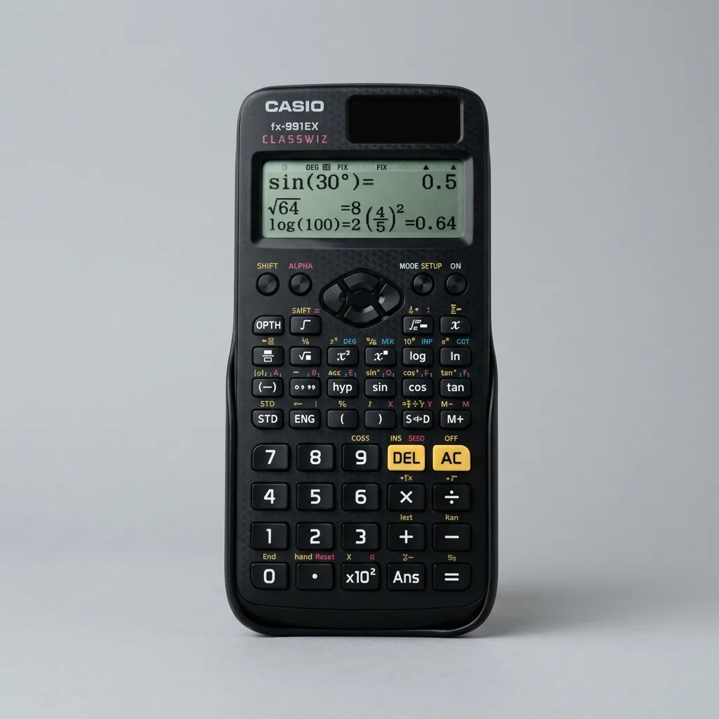
The #1 recommended scientific calculator for board exams, math, and physics.
As an Amazon Associate we earn from qualifying purchases.
Welcome to Class XII Mathematics: Linear Programming. This chapter forms a core structural component of the math syllabus, designed to build analytical rigor and key formula models.
Use the detailed subtopic guide below to review standard definitions, key mathematical rules, and study guidelines.
This comprehensive study guide for Linear Programming is designed for Class XII students following the CBSE and NCERT Mathematics curriculum. It covers 4 key subtopics including Linear Programming problems mathematical formulation, Graphical method for solving LP in two variables, Feasible and infeasible boundary regions, and 1 more essential concepts. Whether you are preparing for school examinations, CBSE board exams, or competitive tests, this resource provides everything you need to build a strong conceptual foundation and achieve mastery.
The chapter includes 1 key formulas and equations, 1 fully worked step-by-step example problems, interactive practice exercises across 9 difficulty categories, timed mock quizzes, and downloadable worksheets. Each topic is explained with detailed concept definitions, mathematical representations, and expert study guidelines to help you understand not just the "how" but the "why" behind every formula and method.
Mathematics is a subject that rewards consistent practice and conceptual clarity over rote memorization. As you work through this chapter on Linear Programming, focus on understanding the underlying principles first, then gradually increase problem difficulty. Use the practice sections to identify and strengthen weak areas, and refer to the common mistakes section to avoid the pitfalls that most students encounter.
By the end of studying Linear Programming for Class XII, you will have developed proficiency in the following learning outcomes as outlined by the NCERT syllabus:
Formulate constraint systems for profit-maximization LP problems.
Graph constraint lines and shade feasible overlap zones.
Evaluate corner points of bounded regions to locate optimal objective targets.
Before studying Linear Programming, make sure you are comfortable with the following prerequisite concepts. A strong foundation in these areas will help you understand new topics faster and solve problems more confidently:
If any of these prerequisites feel unfamiliar, consider reviewing them first using the Related Chapters section at the bottom of this page. Building a solid base ensures you can tackle Linear Programming with full confidence.
Students often wonder “Where will I use Linear Programmingin real life?” The answer is: everywhere. The mathematical concepts you learn in this chapter have practical applications across science, engineering, technology, medicine, finance, and everyday problem-solving. Here are some notable examples:
Factories maximize output or minimize costs by solving linear programming problems with constraints on labor, materials, and machine time.
Shipping companies minimize delivery costs by optimizing routes and vehicle loads using linear programming algorithms.
Dietitians create minimum-cost meal plans that satisfy all nutritional requirements using LP constraint optimization.
Airlines and hospitals optimize staff schedules to ensure coverage while minimizing overtime costs using LP models.
Understanding the real-world relevance of Linear Programming not only makes learning more engaging but also helps you appreciate how mathematical thinking is a superpower that opens doors in virtually every career path — from engineering and medicine to finance and technology.
Follow these expert study strategies to maximize your understanding and exam performance in this chapter. These tips are specifically tailored for the type of content covered in Linear Programming:
Write out every intermediate step when solving problems. Skipping steps is the most common source of errors in calculation-heavy chapters. Build speed only after achieving consistent accuracy.
After finding your answer, substitute it back into the original equation to verify correctness. This simple habit catches most arithmetic and sign errors before they cost you marks.
Keep a dedicated notebook of mistakes you make during practice. Review it weekly to identify patterns — you will notice the same types of errors recurring and can actively work to eliminate them.
Pro Tip: Consistency beats intensity. Studying Linear Programming for 30 minutes daily is far more effective than cramming for 5 hours before the exam. Use the practice sections below to build muscle memory through regular problem-solving.
Review detailed conceptual explanations, mathematical equations, and guidelines for each subtopic in this chapter:
Formulating a Linear Programming Problem (LPP) involves defining decision variables, constructing a linear objective function to maximize or minimize, and setting up linear inequalities representing constraints.
The graphical method solves LPPs by plotting constraints on a coordinate grid, shading the feasible region, and finding the optimal vertex (corner point) using the Corner Point Theorem.
The feasible region is the common region determined by all constraints, including non-negativity constraints. If no common region satisfies all constraints simultaneously, the problem is infeasible.
To find the optimal solution, identify all vertices (corner points) of the feasible region, calculate the value of the objective function Z at each vertex, and select the maximum or minimum value.
By the end of this chapter, students will be able to master and solve questions on these outcomes:
Formulate constraint systems for profit-maximization LP problems.
Graph constraint lines and shade feasible overlap zones.
Evaluate corner points of bounded regions to locate optimal objective targets.
Target linear function optimized under boundary constraints.
[From Three Dimensional Geometry] Vector form of line passing through a parallel to b.
[From Three Dimensional Geometry] Distance between skew lines.
[From Probability] Probability of event A occurring given that event B has occurred.
[From Probability] Inverse conditional probability updates.
Solve trigonometric, exponential, logarithmic, and root functions for standard algebraic values.
Deterministic Mathematical Simulation Engine • Client-Side Computation
Solve trigonometric, exponential, logarithmic, and root functions for standard algebraic values.
| Parameter | Value | Unit |
|---|---|---|
| Value (X) | 45 | — |
| Function | sin | — |
| Metric | Calculated Output |
|---|---|
| Function Output | 0.707 |
MATH SOLVER RUNNING:
 [Inputs] ──► [Mathematical Formula] ──► [Outputs]
  Processed elements successfully.
📚 Level up by completing practice sets.
100% Mastery
No weak areas logged!
Simple algebraic checks with hints and solutions enabled.
Standard curriculum queries matching board exam templates.
Complex math application questions with numeric inputs.
5 mixed questions with a ticking clock to evaluate speed.
Specialized assessment matching the printed worksheets.
Strict 10-question chapter exam. Hints are disabled.
Combines prerequisite concepts and related chapter formulas.
Original questions from previous year CBSE board exams.
High-order logical problems matching Olympiad standards.
Test your math skills with this 5-question chapter mock exam. A live ticking clock will monitor your performance.
Review and solve 10 real Board paper questions from the 16 mock sample sets matching Linear Programming.
Minimize and maximize Z = 600x + 400y Subject to the constraints: x + 2y ≤ 12; 2x + y ≤ 12; 4x + 5y ≤ 20; x≥ 0; y ≥ 0 by graphical method
Solution of LPP To maximise Z = 4x + 8y subject to constraints : 2x + y ≤ 30, x + 2y ≤ 24, x ≥ 3, y ≤ 9, y ≥ 0 is
Solve the following problem graphically: Minimise and Maximise Z = 3x + 9y subject to the constraints: x + 3y ≤ 60; x + y ≥ 10; x ≤ y; x ≥ 0, y ≥ 0
Maximise Z = 8x + 9y subject to the constraints given below : 2x + 3y ≤ 6; 3x - 2y ≤ 6; y ≤ 1; x, y ≥ 0
The feasible region of a ∠PR is given as follows: (i) Write the constraints with respect to the above in terms of x and y. (ii) Find the coordinate of B and C and maximize, z = x + y.
Feasible region is the set of points which satisfy
Feasible region (shaded) for a LPP is shown in the given figure. The maximum value of the Z = 0.4x + y is
Minimise Z = 13x - 15y subject to the constraints x + y ≤ 7, 2x - 3y + 6 ≥ 0, x ≥ 0 and y ≥ 0.
Solve the following LPP graphically: Maximise Z = 3x + 4y Subject to x + y ≤ 4, x ≥ 0 and y ≥ 0.
Minimize and maximize Z = 5x + 2y subject to the following constraints: x - 2y ≤ 2, 3x + 2y ≤ 12, -3x + 2y ≤ 3, x ≥ 0, y ≥ 0
Recognizing and eliminating common errors is a key step to scoring high marks in school and board exams:
Solving additions or subtractions before evaluating parentheses, exponents, divisions or multiplications.
Doing addition/subtraction to only one side of the equation when rearranging terms.
Misplacing the decimal dot when dividing by factors of ten.
Commit core formulas to memory and write them down before solving problems.
Verify that all physical parameters use compatible measurement units.
Use our interactive calculator solvers to verify manually computed decimal answers.
Ensure all prerequisite concepts are fully understood before working on advanced calculations.
Always check equations step-by-step to avoid simple sign and arithmetic errors.
Resolve equations using alternative methods (e.g., check quadratic roots by plugging them back into ax² + bx + c), verify decimals using scientific solvers, and review step-by-step worked calculations.
Trigonometry is used in architecture, mechanics and navigation. Quadratic equations model rocket trajectories and profit boundaries. Basic arithmetic and fractions are applied in accounting, budgeting and lab chemistry.
Check out these related chapters and pre-requisites to strengthen your analytical foundation:
[Adjacent Chapter] Convert line equations between vector and Cartesian formats.
[Adjacent Chapter] Calculate conditional probabilities.
Prove if a relation is reflexive, symmetric, and transitive, classifying it as equivalence.
Use these related calculator solvers to verify variables and double check homework steps:
Solve trigonometric, exponential, logarithmic, and root functions for standard algebraic values.
Perform arithmetic operations on fractions: add, subtract, multiply, and divide two fractions. Simplifies the results dynamically and provides decimal equivalencies.
Select any key syllabus topic below to open its detailed learning guide, worked models, and study guidelines.
Learn the easiest ways to simplify fractions. Master finding the Greatest Common Divisor (GCD) and reducing fractions to their simplest form with worked examples.
Demystify mathematical sequences. Learn to identify arithmetic and geometric progressions, calculate common differences/ratios, and find the nth term.
Learn the math behind ratios and proportions. Master scaling values, dividing amounts by ratios, and solving proportions using cross-multiplication.
Generate and print a beautiful chapter worksheet complete with key equations, problems, and dedicated writing spaces.
1. Minimize and maximize Z = 600x + 400y Subject to the constraints: x + 2y ≤ 12; 2x + y ≤ 12; 4x + 5y ≤ 20; x≥ 0; y ≥ 0 by graphical method
2. Solve the following problem graphically: Minimise and Maximise Z = 3x + 9y subject to the constraints: x + 3y ≤ 60; x + y ≥ 10; x ≤ y; x ≥ 0, y ≥ 0
3. Maximise Z = 8x + 9y subject to the constraints given below : 2x + 3y ≤ 6; 3x - 2y ≤ 6; y ≤ 1; x, y ≥ 0
4. The feasible region of a ∠PR is given as follows: (i) Write the constraints with respect to the above in terms of x and y. (ii) Find the coordinate of B and C and maximize, z = x + y.
5. Minimise Z = 13x - 15y subject to the constraints x + y ≤ 7, 2x - 3y + 6 ≥ 0, x ≥ 0 and y ≥ 0.